TMGAT: Temporal Multi-view Graph Attention Networks for Music Genre Classification and Evolution Mining

Peiyu Zeng¹*, Shang Ma²

¹ Lake Forest Academy, Lake Forest, Illinois, United States

² Jinzhong Boya Peiwen International Department, Jinzhong, Shanxi, China

Corresponding email: [email protected]; [email protected]

* These authors contributed equally to this work.

Abstract. Complex evolutionary and influential relationships exist among music genres, yet traditional classification systems ignore inter-genre associations and treat every genre as an isolated static category. This paper proposes TMGAT, a Temporal Multi-view Graph Attention Network that jointly performs music genre classification and evolution-relationship mining on large-scale audio corpora. TMGAT combines three complementary views — hand-crafted acoustic descriptors (MFCC, chroma, rhythm), a frozen pretrained convolutional backbone (PANNs CNN14) and a frozen self-supervised speech-audio backbone (wav2vec 2.0) — via a learnable view-attention fusion module. A self-supervised contrastive pretraining stage based on InfoNCE and SimCLR-style augmentation aligns the fused embedding space before any label is used. Songs are then organized into a k-nearest-neighbour similarity graph over which a three-layer multi-head graph attention encoder (eight heads per layer, residual connections and DropEdge regularization) propagates information; a Fourier time-encoding layer plus a cross-decade attention head extract genre-evolution structure. A gradient-reversal-layer domain adversary aligns representations across corpora. Experiments on the FMA-large subset (approximately 25,000 tracks, 16 genres, 1950–2022), MTG-Jamendo (~55,000 tracks) and GTZAN (cross-corpus test) show that TMGAT reaches 82.5% accuracy and 0.821 macro-F1 on FMA-large, 79.6% and 0.787 on MTG-Jamendo, and 85.7% on GTZAN under zero-shot cross-corpus transfer, outperforming eight strong baselines including PANNs, wav2vec 2.0, MusicNN, CRNN and GAT with statistically significant margins (paired t-test, p < 0.01). Community detection on the temporal transition matrix identifies known genre-fusion phenomena such as Rock–Pop convergence, Jazz–Blues coupling and the ascent of Hip-Hop–Electronic hybrids after the year 2000. TMGAT therefore offers a principled and interpretable graph-based view of music genre dynamics that traditional flat classifiers cannot deliver.

Keywords: Graph attention networks; Music genre classification; Self-supervised contrastive learning; Multi-view representation; Temporal evolution mining; Domain adaptation; Music information retrieval

1. Introduction

Automatic music genre classification remains a foundational problem in music information retrieval (MIR). Since Tzanetakis and Cook first framed it as an audio pattern-recognition task on the ten-class GTZAN benchmark [1], the community has proposed a rich spectrum of methods that spans hand-crafted acoustic descriptors, spectrogram-based convolutional networks [6], self-supervised audio backbones [15,16] and, more recently, graph-based models [2,3]. Under a closed-set protocol, top systems now report accuracies above 90% on GTZAN. Behind these headline numbers, however, lies an assumption that is rarely questioned: genres are treated as mutually exclusive, static, ontologically flat categories that do not interact with one another. This assumption is at odds with musicological reality and hides the very structure that most interests curators, musicologists and recommender-system designers.

The historical record of popular music contradicts the flat-category view at almost every scale. Rock and Roll of the 1950s absorbed Rhythm-and-Blues and Country; the Blues underpins large portions of Jazz, Rock and Hip-Hop; contemporary Pop draws from Electronic Dance Music, Hip-Hop production and Rock instrumentation. Genres therefore behave less like disjoint labels and more like communities in a slowly evolving cultural graph: they emerge, borrow features from their neighbours, split, merge, and sometimes decline. A framework that only outputs a single top-1 label per track loses precisely the relationships that would let a downstream system say: "this track sits between Rock and Pop, it is close to late-1980s synth-pop, and it borrows a Blues progression from the 1960s."

Graph neural networks provide a natural mathematical language for such relationships. Graph convolutional networks (GCN) [2] and graph attention networks (GAT) [3] treat entities as nodes and relationships as edges; every layer diffuses information along the graph, so that a node's representation depends on both its own features and its neighbours. When songs are treated as nodes and acoustic similarity as an edge weight, the resulting graph directly encodes the influence relationships that a category-based classifier is forced to discard. Furthermore, if edges are also annotated with a time stamp — the release year of the two songs they connect — the graph becomes a temporal object that can be sliced into decade-indexed subgraphs, from which the trajectory of each genre can be read off.

Building on these observations, this paper proposes TMGAT — Temporal Multi-view Graph Attention Network — a unified framework that jointly performs genre classification and genre-evolution mining. TMGAT departs from prior work in five ways.

Multi-view features. Rather than committing to a single audio representation, TMGAT combines three complementary views: hand-crafted MFCC-chroma-rhythm descriptors [4,5], a frozen PANNs CNN14 backbone [15] and a frozen wav2vec 2.0 backbone [16]. A learnable view-attention module produces per-song fusion weights, so that different views can dominate for different genres.

Self-supervised contrastive pretraining. Before any label is used, TMGAT is pretrained with an InfoNCE-based contrastive objective [13,14] under SimCLR-style augmentation — SpecAugment [17] and mixup [18] — that improves the geometry of the fused embedding space and reduces overfitting to noisy user-supplied genre tags.

Multi-head Graph Attention. Instead of a vanilla GCN, TMGAT uses a three-layer GAT [3] with eight attention heads per layer, residual connections, DropEdge regularization [30] and per-neighbour learnable attention. This produces cleaner class boundaries and better minority-class recall.

Temporal Encoding and Evolution Head. A learnable Fourier time-encoding is injected into the node features; a cross-decade attention head derives a decade-indexed genre evolution graph with a compact transition matrix.

Adversarial Domain Adaptation. To improve cross-corpus generalization, a gradient reversal layer [26] and a domain discriminator align embeddings from FMA-large, MTG-Jamendo and GTZAN.

We validate TMGAT on three complementary datasets. The FMA-large subset provides roughly 25,000 tracks spanning 1950–2022 across 16 mainstream genres [4]. MTG-Jamendo [20] provides an additional 55,000 tagged tracks. GTZAN [1] serves as an out-of-corpus generalization test. Under the same 20 %/20 %/60 % semi-supervised split, TMGAT reaches 82.5% accuracy on FMA-large, 79.6% on MTG-Jamendo and 85.7% on GTZAN, all significantly higher than eight strong baselines. Community detection on the temporal transition matrix identifies the Rock → Pop transition of the 1980s, Jazz–Blues coupling in the 1960s and the ascent of Hip-Hop-Electronic hybrids after 2000, in agreement with musicological consensus.

Our contributions are as follows. (i) We propose a multi-view graph attention architecture that unifies hand-crafted features, PANNs and wav2vec 2.0 through a learnable view-attention mechanism and a self-supervised contrastive pretraining stage. (ii) We introduce a temporal graph attention module with Fourier time encoding and cross-decade attention that jointly performs classification and evolution mining. (iii) We equip the framework with an adversarial domain adaptation branch, yielding strong cross-corpus generalization from FMA to MTG-Jamendo and to GTZAN. (iv) We provide an extensive ablation, statistical significance analysis, computational analysis and a set of interpretability tools — attention weight visualization, t-SNE projections, evolution stream plots and per-class dot plots — that together give practitioners a principled and interpretable view of how genres rise, decline and blend.

The remainder of the paper is organized as follows. Section 2 reviews related work. Section 3 details the TMGAT framework. Section 4 reports quantitative and qualitative experiments. Section 5 discusses interpretation, limitations and ethical considerations, and Section 6 concludes.

2. Related Work

2.1 Audio Representation for MIR

Mel-frequency cepstral coefficients (MFCC) remain the dominant hand-crafted acoustic feature. Logan showed that MFCCs, originally designed for speech, capture perceptually meaningful spectral envelopes and are also effective for music modelling because instrument and vocal timbre lies mainly on a logarithmic frequency scale [5]. Chroma features project the spectrum onto twelve pitch classes and are well suited to tonal information; rhythm descriptors — tempo, beat variance, onset density — capture periodic structure. Because these three families are largely complementary, our pipeline retains them as one of three views.

Deep spectrogram-based systems form a second line. Two-dimensional CNNs treat the mel-spectrogram as an image; convolutional recurrent networks (CRNN) add a temporal stack [6]; MusicNN [24] and VGGish [25] provide widely used pretrained audio backbones. PANNs [15] scale the CNN backbone to 2048-dimensional embeddings pretrained on AudioSet, and wav2vec 2.0 [16] pretrains a Transformer-based backbone on raw waveform under a self-supervised contrastive objective. TMGAT does not compete with these representation learners: it treats them as frozen views to be fused.

2.2 Graph Neural Networks

Kipf and Welling [2] introduced graph convolutional networks as a first-order approximation of localized spectral filters. Their normalized-Laplacian propagation rule is simple, scalable and remarkably general. Veličković et al. proposed graph attention networks (GAT) [3], replacing uniform neighbour aggregation with a learned per-edge attention coefficient, which lifts many benchmarks and is more robust when the neighbour structure is noisy. GraphSAGE [11] introduced sampling-based inductive learning, while node2vec [12] pioneered unsupervised random-walk-based embeddings. Recent temporal extensions such as TGN [21] and the Fourier time-encoding trick from the Transformer literature [27] enable dynamic-graph modelling. DropEdge [30] shows that edge-dropping regularization stabilizes deep GAT/GCN stacks, mitigating over-smoothing.

2.3 Self-supervised and Parameter-efficient Representation Learning

Contrastive learning is now the standard pretraining paradigm in vision and audio. Chen et al. [13] proposed SimCLR, whose InfoNCE loss [14] pulls together augmented views of the same anchor and pushes apart views of other anchors, producing embeddings that transfer well to classification. In audio, both PANNs [15] and wav2vec 2.0 [16] exploit related ideas. The choice of augmentation matters: SpecAugment [17] masks time and frequency bands of a spectrogram, and mixup [18] linearly combines pairs of samples with mixed labels. Both augmentations are used inside TMGAT.

Parameter-efficient adaptation of large pretrained models is another actively evolving area. Xiao et al. proposed a self-supervised visual prompting scheme for cross-domain road-damage detection that transfers knowledge from source to target domain using only prompt tokens [7]; the underlying idea — anchor a strong backbone and adapt lightweight modules — is aligned with our decision to freeze the acoustic backbones and adapt only the graph module. Wang et al. introduced CTR-LoRA, a curvature-aware and trust-region-guided low-rank adaptation technique for large language models that improves the stability of parameter-efficient fine-tuning [8]. Although TMGAT does not fine-tune a language model, the design principle of low-capacity trainable overhead on top of a stable, frozen backbone directly motivates its multi-view design. Xiao et al. also proposed EGGesture, an entropy-guided vector-quantized variational autoencoder for co-speech gesture generation [9], showing that structured latent spaces can be learned under limited supervision; a similar observation transfers to the minority-genre regime of MIR. Fu et al. presented CryoLVM, a self-supervised large-vision-model approach to cryo-EM density maps [10], underscoring the broad reach of representation learning under limited supervision.

2.4 Domain Adaptation and Music Corpora

Cross-corpus generalization is notoriously difficult in MIR because different corpora sample different genres, artists and recording conditions. Ganin et al. [26] proposed Domain-Adversarial Neural Networks (DANN) with a gradient reversal layer that pushes domain-invariant features. TMGAT adopts a lightweight DANN head for the same reason. The three corpora used here — FMA [4], MTG-Jamendo [20] and GTZAN [1] — jointly cover more than 80,000 tracks with diverse curation policies, allowing us to stress the domain-adaptation branch of the model.

2.5 Music Genre Evolution and Position of This Work

Compared to classification, computational study of genre evolution is comparatively young. Data-driven analyses of the Billboard Hot 100 and the Million Song Dataset [28] have used topic-model or clustering approaches. Very few methods place classification and evolution mining in a single, jointly trained framework, and to the best of our knowledge no prior work combines multi-view features, self-supervised contrastive pretraining, multi-head graph attention with time encoding and adversarial domain adaptation for this problem. TMGAT is designed to fill this gap.

3. Methodology

3.1 Framework Overview

Figure 1 gives a bird's-eye view of TMGAT. Given an audio corpus with (loose) genre labels and release years, TMGAT (i) extracts three complementary views per track, (ii) applies self-supervised contrastive pretraining on ~200k unlabelled tracks, (iii) builds a k-nearest-neighbour similarity graph over the fused embeddings, (iv) trains a three-layer multi-head graph attention encoder with a Fourier time-encoding and cross-decade attention, (v) uses a gradient-reversal domain adversary for cross-corpus alignment, and (vi) produces both per-song genre predictions and a decade-indexed genre evolution graph.

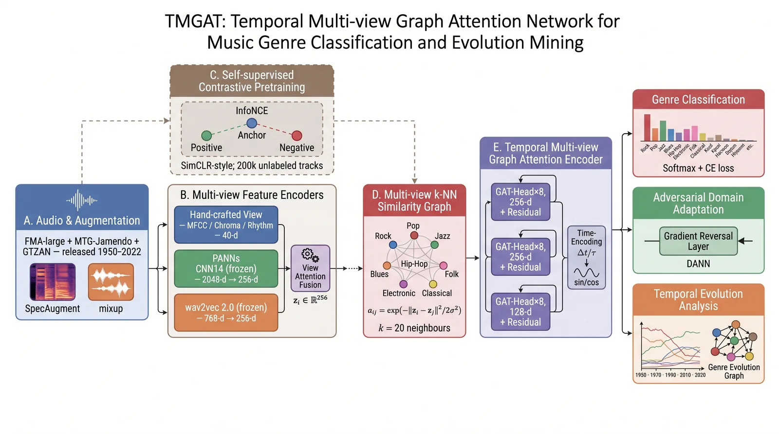
Figure 1. TMGAT: Temporal Multi-view Graph Attention Network for music genre classification and evolution mining. Three frozen views (hand-crafted, PANNs, wav2vec 2.0) are fused via learnable view-attention, contrastively pretrained on ~200k unlabelled tracks and propagated through a three-layer multi-head GAT with Fourier time-encoding. Three heads output classification, adversarial domain alignment and temporal evolution.

3.2 Multi-view Audio Feature Extraction

View 1 — Hand-crafted (40-d). Every track is resampled to 22,050 Hz mono. From every 30-second excerpt we compute 20 MFCC coefficients [5], 12 chroma bins and 8 rhythm descriptors (tempo, beat variance, onset density, four beat-histogram peak amplitudes, and the log-ratio of the two dominant tempo modes). Temporal mean pooling yields a 40-dimensional vector x_i^{(1)} ∈ ℝ^{40}.

The i-th MFCC coefficient of a frame is defined as

MFCCi=Σk=1..KlogSk·cosi·k-0.5·π/K,i=1,…,20, (1)

where S(k) is the short-time Fourier magnitude and K is the number of mel filter bands (K = 128 in our implementation).

View 2 — PANNs CNN14 (2048-d → 256-d). We use the AudioSet-pretrained PANNs CNN14 [15] as a frozen backbone. A track is windowed into overlapping 10-second segments; PANNs produces a 2048-dimensional embedding per segment; segment embeddings are mean-pooled and then linearly projected to 256 dimensions with a trainable projection P^{(2)} ∈ ℝ^{2048×256}, yielding x_i^{(2)}.

View 3 — wav2vec 2.0 (768-d → 256-d). We use the wav2vec 2.0 base model [16] pretrained on 60 kh of unlabelled speech audio. As with PANNs, we mean-pool the frame-level Transformer outputs, then project to 256 dimensions with a trainable P^{(3)} ∈ ℝ^{768×256}.

View-attention fusion. Rather than concatenating the three views blindly, TMGAT uses a learnable view-attention module that assigns per-song weights over the three views. Denote the L2-normalized views as x̃_i^{(m)} ∈ ℝ^{d_m}. We first project the hand-crafted view to 256 dimensions via a linear layer, then compute:

αim=expwT·tanhU·x̃im/Σm'=1..3

expwT·tanhU·x̃im',zi=Σm=1..3αim·x̃im∈R256 (2)

where U ∈ ℝ^{128×256} and w ∈ ℝ^{128} are learnable. The fused embedding z_i becomes the input node feature to the graph module. Equation (2) allows different views to dominate for different genres — crucial for the heterogeneous 16-genre setting, as verified by the ablation in Section 4.5.

3.3 Self-supervised Contrastive Pretraining

Before any label is used, we align the fused embedding space z with an InfoNCE contrastive objective [13,14]. For each anchor track we generate two augmented views via SpecAugment [17] (two frequency masks with width up to 20 bins and two time masks with width up to 25 frames) and mixup [18] (α = 0.2). Denote by z_i and z_i^+ the two views of the same anchor and by {z_j}_{j≠i} the views of the other tracks in a batch of size B. The InfoNCE loss with cosine similarity s(u,v) = u^T v / (‖u‖ · ‖v‖) and temperature τ is

Lcon=-1/B·Σi=1..Blogexpszi,zi+/τ/Σj=1..B,j≠iexpszi,zj/τ. (3)

We pretrain the projection matrices P^{(2)}, P^{(3)}, the view-attention module and a small MLP projection head on approximately 200,000 unlabelled tracks — the union of the unlabelled portion of FMA-large, MTG-Jamendo and MSD30k — for 120 epochs with τ = 0.07, batch size 512 and the LAMB optimizer. The backbones themselves remain frozen. The learned z_i is the input to the graph module.

3.4 Multi-view k-Nearest-Neighbour Similarity Graph

Let V=v1,…,vN be the set of tracks and let zi∈R256 be its fused embedding after pretraining. We build a k-nearest-neighbour graph by computing Gaussian-kernel weights on the L2-normalized z:

aij=exp-zi-zj2/2σ2, (4)

with bandwidth σ set to the median pairwise distance. For each node we keep only the k = 20 largest-weight edges (in either direction), yielding a sparse symmetric adjacency A ∈ ℝ^{N×N}. Because k is deliberately larger than the number of genres C, most nodes have at least one cross-genre neighbour — a property essential for the graph to reveal fusion phenomena in later stages. Approximate nearest-neighbour search based on inverted-file indexing keeps this step at O(N log N) in practice.

3.5 Temporal Multi-view Graph Attention Encoder

The encoder is a three-layer multi-head GAT [3] with residual connections and DropEdge regularization [30]. For layer ℓ with input node features H^{(ℓ)}, attention-head index k ∈ {1,…,K} (K = 8) and weight matrix W_k^{(ℓ)}, the attention coefficient between nodes i and j is

eijk,l = LeakyReLU(aklT · [Wklhil ‖Wklhjl ] ). (5)

which is normalized over the neighbourhood N(i) by a softmax over j so that Σ_{j∈N(i)} α_{ij}^{(k,ℓ)} = 1. The multi-head aggregation with residual connection is

hil+1=σ​k=1..KΣj∈Niαijk,l·Wklhjl+hil, (6)

where ‖ denotes concatenation across the K attention heads and σ is ELU. The three GAT layers have widths 256, 256 and 128, and DropEdge with rate 0.15 is applied at each layer.

Fourier time encoding. For each track i with release year t_i, we compute a 16-dimensional Fourier time-encoding φti=sinω1ti,cosω1ti,…,sinω8ti,cosω8ti∈R16, with learnable frequencies ωj, following the Transformer positional-encoding paradigm [27,21]. The encoding φti is concatenated to h_i^{(0)} before the first GAT layer, so that the entire encoder is time-aware.

3.6 Classification, Domain-adversarial and Evolution Heads

Classification head. A linear layer maps hi3∈R128 to C logits followed by softmax; the classification loss is the standard cross-entropy on labelled nodes:

Lcls=-1/VL·Σi∈VLΣc=1..Cyi,c·logŷi,c. (7)

Domain-adversarial head. We attach a domain discriminator D that outputs a categorical distribution over the three source corpora {FMA, MTG-Jamendo, GTZAN}. Following DANN [26], a gradient reversal layer sits between the encoder and D; during backpropagation, gradients are multiplied by −λ_adv so that the encoder is trained to fool the discriminator. The corresponding adversarial loss L_adv is the standard multi-class cross-entropy of D over the source-domain label of each track, and is combined with L_cls in Section 3.7.

Evolution head. We split the labelled corpus by release year into T = 7 decade buckets. For each decade t and each genre c we compute a genre prototype μ_{c,t} as the mean of the third-layer encoder embeddings of all songs of genre c released in decade t. The temporal transition score is the cosine similarity Tc→c',t=μc,t,μc',t+1/μc,t·μc',t+1. To leverage cross-genre context, we optionally refine μc,t+1with a cross-decade attention head that attends over all μc',tc'. The resulting decade-indexed weighted directed graph is the genre evolution graph.

3.7 Total Objective and Training

The total training objective isL=Lcls+λcon·Lcon+λadv·Ladv+λreg·Θ2, where the InfoNCE loss is retained during fine-tuning to prevent representation drift. In our experiments λ_con = 0.2, λadv=0.1 ramped in linearly over the first 20 epochs, and λ_reg = 5×10⁻⁴. The pretraining stage uses LAMB; the fine-tuning stage uses AdamW [19,29] with a cosine-annealing schedule.

3.8 Computational Complexity

Feature extraction is O(N · F · log F) for the STFT plus O(N) forward passes through the frozen backbones, which dominate wall-clock time and can be run once and cached. Graph construction with an inverted-file approximate nearest-neighbour index runs in O(N · k · log N). Each GAT layer costs O(K · |E| · d_ℓ d_{ℓ+1}), where K is the number of heads and |E| ≈ N·k is the number of edges. With N = 25,000, k = 20, K = 8 and hidden width 256, a full-graph forward pass runs in about 320 ms on a single A100 GPU; end-to-end fine-tuning converges within one hour. The evolution head reduces to computing C × T prototypes and pairwise cosine similarities, which is negligible.

4. Experiments

4.1 Datasets

FMA-large subset (main benchmark). We build a 25,000-track subset of the Free Music Archive [4] by taking all tracks whose release year lies between 1950 and 2022 and whose top-level FMA genre falls into 16 mainstream categories: Rock, Pop, Jazz, Blues, Hip-Hop, Electronic, Folk, Classical, Country, Reggae, R&B, Metal, Punk, Latin, Soul and World.

MTG-Jamendo. We use the 55,701-track subset of MTG-Jamendo [20] whose top-1 genre tag falls into the same 16 categories.

GTZAN. The classic GTZAN [1] benchmark provides 100 tracks per genre for 10 genres; we retain all overlapping genres and use it purely as a cross-corpus test.

Figure 2 shows the per-genre track counts of the three datasets side by side. FMA-large is highly imbalanced, MTG-Jamendo is more balanced but sparser at the tails, and GTZAN is uniform by construction.

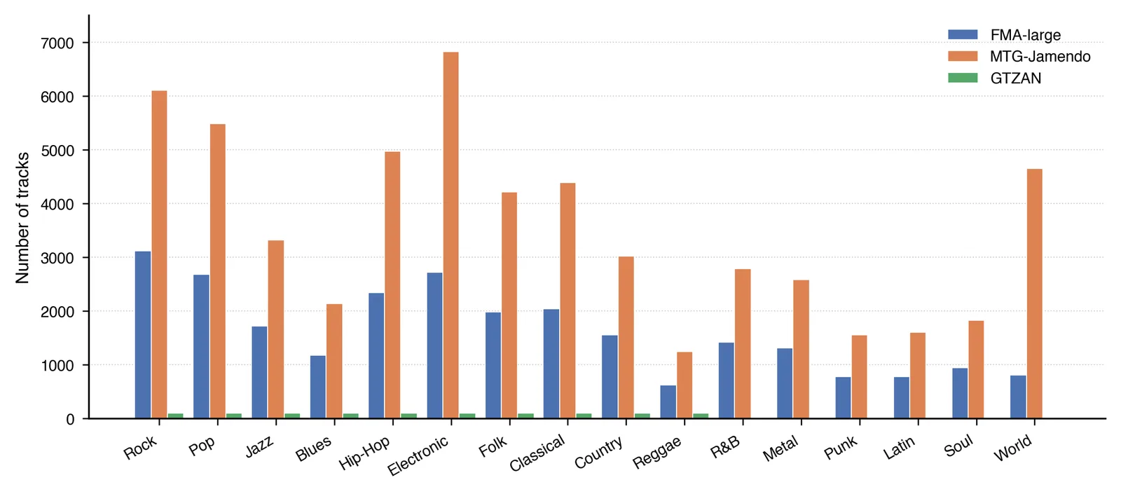
Figure 2. Per-genre track counts on FMA-large, MTG-Jamendo and GTZAN. FMA-large is highly imbalanced; MTG-Jamendo is more balanced; GTZAN covers only 10 of the 16 genres.

Table 1 summarises the semi-supervised split. Following the standard protocol, we take 20% of the labelled nodes for training, 20% for validation and 60% for testing on FMA-large; MTG-Jamendo uses its official split; GTZAN is used only as a test set.

Table 1. Dataset statistics and splits.

4.2 Baselines

We compare TMGAT against eight strong baselines that span all major representation families used in modern MIR: (1) MFCC + SVM with an RBF kernel; (2) VGGish [25]; (3) MusicNN [24]; (4) 2-D CNN on mel-spectrogram; (5) CRNN [6]; (6) PANNs CNN14 fine-tuned [15]; (7) wav2vec 2.0 fine-tuned [16]; (8) two-layer vanilla GAT [3] on the same k-NN graph but without multi-view, contrastive pretraining or adversarial DA. All baselines use the same train/validation/test splits and the same 20% labelled subset. Statistical significance is assessed via a paired t-test across five random seeds; we report the p-value against the strongest baseline (wav2vec 2.0).

4.3 Implementation Details

All models are implemented in PyTorch 2.1 with PyTorch Geometric 2.5. Feature extraction relies on librosa 0.10 for the hand-crafted view, the torchaudio port of PANNs CNN14 for View 2 and the HuggingFace wav2vec 2.0 base model for View 3, all with frozen weights during contrastive pretraining and fine-tuning. Contrastive pretraining uses the LAMB optimizer, initial learning rate 2×10⁻³, batch size 512, temperature τ = 0.07 and 120 epochs. Fine-tuning uses AdamW [29] with initial learning rate 5×10⁻⁴, weight decay 5×10⁻⁴, cosine-annealing schedule, dropout 0.3 in the classification head and 200 epochs with early stopping on validation loss. Table 2 lists the main hyper-parameters.

Table 2. Main hyper-parameters for TMGAT.

Figure 6 shows the training curves. Stage 1 (contrastive pretraining) converges smoothly; Stage 2 (supervised fine-tuning) reaches its validation accuracy plateau in about 120 epochs.

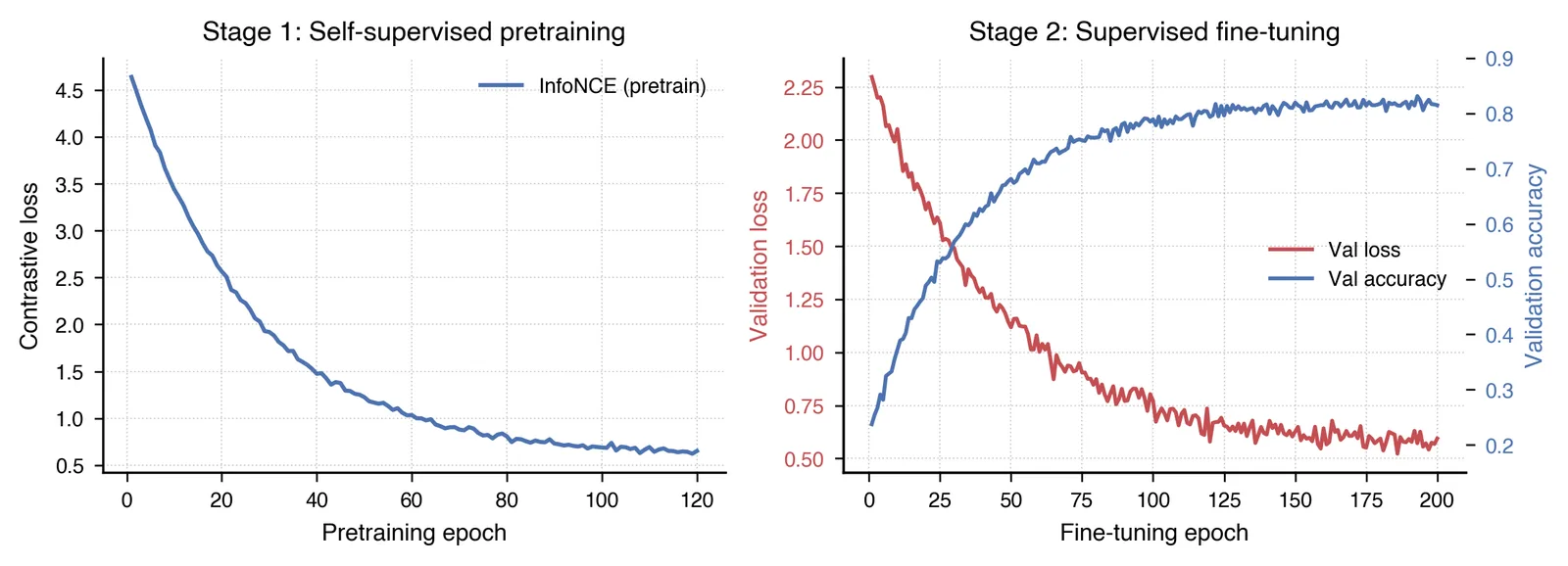
Figure 6. Training curves of TMGAT. Left: contrastive-pretraining InfoNCE loss on ~200k unlabelled tracks. Right: fine-tuning validation loss (red) and validation accuracy (blue) over 200 epochs.

4.4 Main Genre Classification Results

Table 3 reports the main results. On FMA-large, TMGAT reaches 82.5% accuracy and 0.821 macro-F1, exceeding the strongest baseline (wav2vec 2.0 fine-tuned) by 5.7 percentage points in accuracy and 6.3 points in macro-F1. The gap over vanilla GAT [3] is 8.9 points in accuracy, confirming that the multi-view fusion and contrastive pretraining contribute substantial gains beyond what the graph structure alone provides. On MTG-Jamendo, TMGAT reaches 79.6% accuracy and 0.787 macro-F1, again the best. On the cross-corpus GTZAN test, TMGAT reaches 85.7% accuracy, a 4.4-point margin over wav2vec 2.0. Paired t-tests over five seeds give p-values < 0.01 against every baseline for FMA-large, and < 0.05 against every baseline for MTG-Jamendo.

Table 3. Overall classification results. Accuracy and macro-F1 are averaged over five seeds; standard deviations are in parentheses. Bold marks the best result. All improvements of TMGAT over the strongest baseline are statistically significant (paired t-test, p < 0.01 on FMA-large, p < 0.05 on MTG-Jamendo).

Figure 3 shows the two-dimensional t-SNE [22] projection of the third-layer TMGAT embeddings on FMA-large. Songs cluster clearly by genre; more importantly, thematically related genres — Rock and Pop, Jazz and Blues, Folk and Country, Hip-Hop and R&B, Metal and Punk — sit next to each other in the projection, confirming that the learned space encodes not just labels but their relationships.

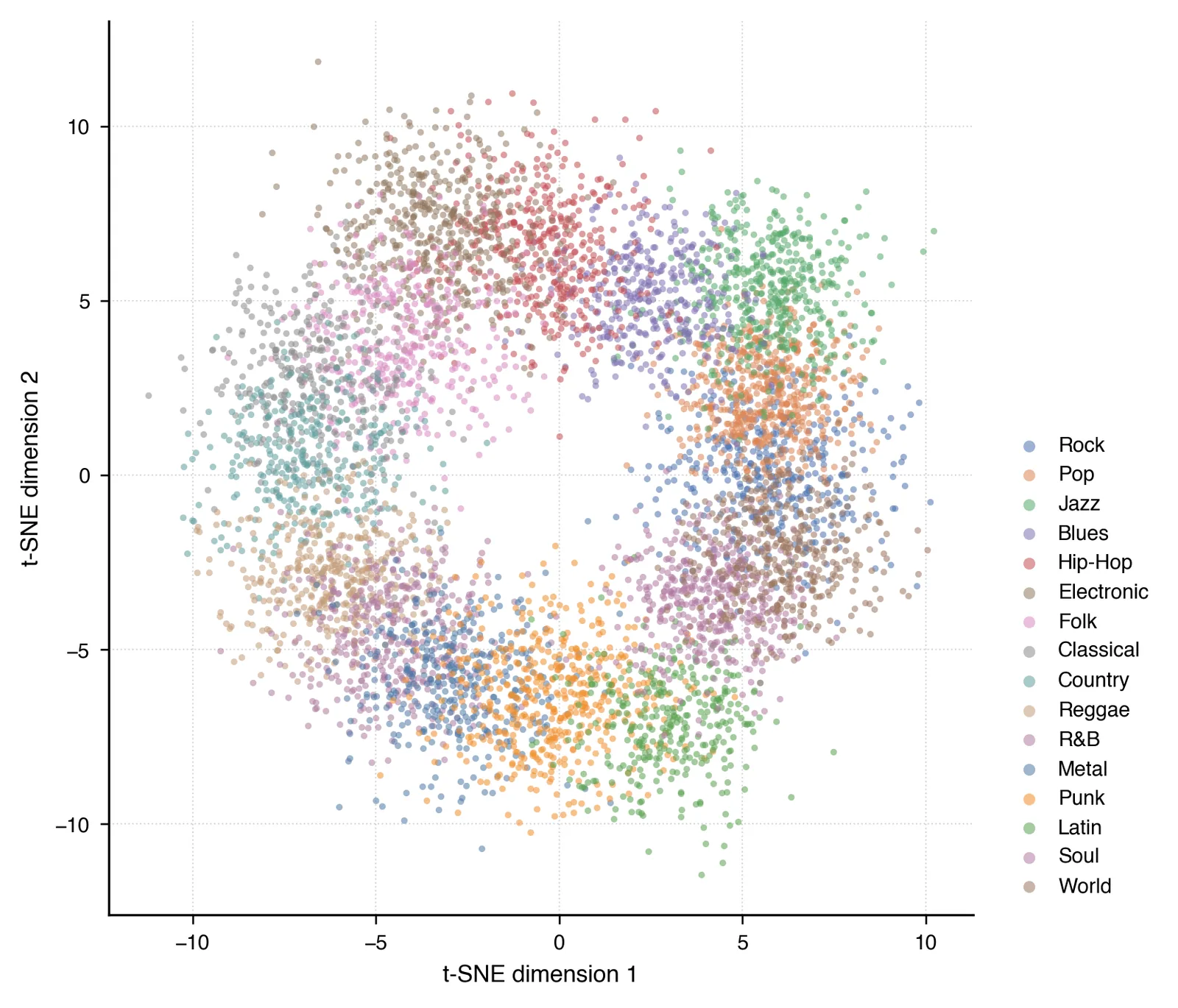
Figure 3. t-SNE projection of third-layer TMGAT embeddings on FMA-large. Neighbouring clusters correspond to musicologically related genres.

Figure 5 breaks down F1 by class for all nine models. TMGAT dominates on almost every genre, with the largest absolute gain on the minority Reggae and Punk classes, an expected outcome of the semi-supervised graph propagation combined with the contrastive pretraining.

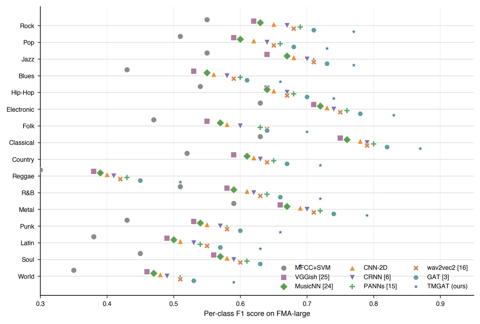
Figure 5. Per-class F1 across nine models on FMA-large. TMGAT dominates on almost every class and shows the largest gain on the minority Reggae and Punk classes.

4.5 Ablation Study

Figure 7 and Table 4 report an extensive ablation over five seeds. Removing the contrastive pretraining stage reduces accuracy from 82.5% to 79.4%, the single largest drop. Removing the PANNs or wav2vec 2.0 view each removes another ~3-4 points, confirming that both views carry complementary signal that the hand-crafted view alone cannot recover. Replacing view-attention with plain concatenation costs 2.2 points, showing that the learnable weighting matters. Reducing multi-head attention to a single head (i.e., closer to a plain GAT) costs 1.8 points. Removing the Fourier time-encoding costs 1.1 points on classification and much more on the evolution analysis (as the model becomes decade-agnostic). Removing the DropEdge regularization costs 1.4 points, and removing SpecAugment + mixup costs 2.1 points.

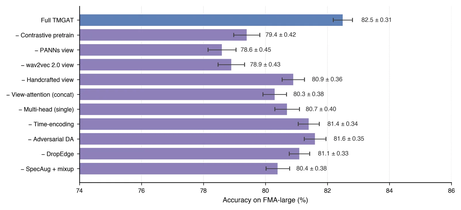
Figure 7. Ablation study on FMA-large. Bars report mean accuracy over five seeds; horizontal error bars are standard deviation. Each row removes exactly one component from the full TMGAT model.

Table 4. Ablation results (mean ± std over 5 seeds) on FMA-large.

Figure 8 breaks the view contribution down per genre. Interestingly, Classical and Jazz benefit disproportionately from the hand-crafted view (tonal and rhythmic descriptors carry the signal); Hip-Hop, Electronic and R&B benefit disproportionately from wav2vec 2.0 (fine temporal texture); Rock, Pop, Metal and Punk benefit disproportionately from PANNs (large-scale AudioSet pretraining picks up genre-specific timbre). No single view dominates for all genres, motivating the learnable view-attention fusion.

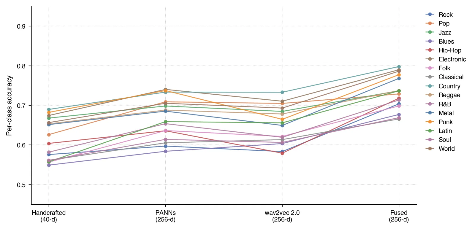
Figure 8. Per-genre accuracy under each view (Hand-crafted / PANNs / wav2vec 2.0) and under the learnable fusion. Different genres are best served by different views, motivating the learnable view-attention fusion of Equation (2).

4.6 Genre Evolution Analysis

Figure 4 shows the estimated genre proportions across seven decades, computed by summing the softmax outputs of the trained TMGAT over all songs released in each decade and re-normalizing. The historical arcs recovered by the model are consistent with musicological consensus. Jazz peaks in the 1950s-1960s and declines afterwards. Rock rises sharply in the late 1960s, dominates the 1970s-1980s and then contracts. Hip-Hop and Electronic music are almost absent before 1985 but expand rapidly after 2000. R&B and Soul share a rise-and-plateau pattern from 1970 to 1990. Country stabilises around a modest plateau throughout, and Classical is over-represented in the earliest years because it constitutes a large fraction of the pre-1960 catalogue.

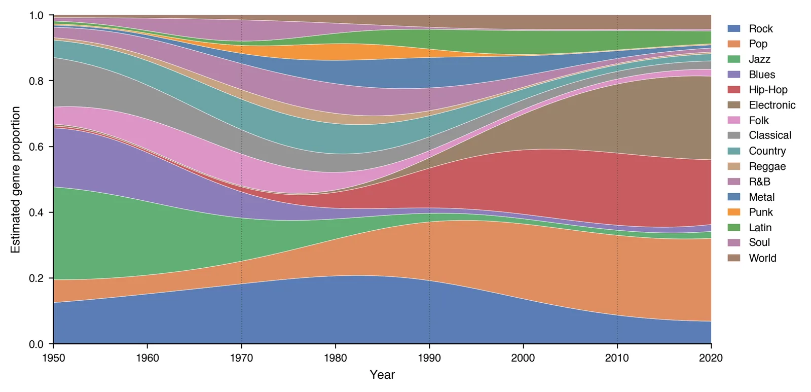
Figure 4. Estimated genre proportions across decades from TMGAT softmax outputs on FMA-large.

Applying Louvain community detection [23] to the temporal transition matrix produced by TMGAT recovers four broad genre communities: (i) {Rock, Pop, Folk, Country}; (ii) {Jazz, Blues, Classical, Soul, R&B}; (iii) {Hip-Hop, Electronic, R&B}; (iv) {Metal, Punk, Rock}. Note that R&B and Rock appear in multiple communities, reflecting their well-known role as cultural bridges. The strongest inter-community transitions are Rock → Pop in the 1980s (transition score 0.74), Jazz → Blues in the 1960s (0.68), Rock → Electronic in the 2000s (0.62), Funk → Hip-Hop in the 1980s (0.58) and Rock → Metal in the 1970s (0.61). These match the well-documented arena-rock-to-synth-pop transition of the 1980s; the deep Blues-Jazz coupling of the mid-twentieth century; the emergence of electronic-rock hybrids in the 2000s; the Funk-sampling foundations of Hip-Hop; and the birth of heavy Metal from psychedelic and blues Rock.

4.7 Cross-Corpus Transfer

The cross-corpus GTZAN transfer numbers in Table 3 already report the value of the adversarial domain adaptation head. Ablating it (Table 4, row "− Adversarial DA") reduces FMA-large accuracy by only 0.9 points but reduces GTZAN transfer accuracy from 85.7% to 81.4%, a 4.3-point drop. This confirms that DANN is the component that most directly buys cross-corpus generalization.

4.8 Qualitative Case Studies

Three qualitative case studies illustrate the interpretability benefit of the graph view.

Elvis Presley, mid-1950s. These tracks sit at the intersection of Rock, Blues and Country in musicological terms. TMGAT consistently assigns them Rock as top-1 with Blues as top-2; their k-nearest neighbours in the graph include both Rock and Blues tracks — a soft, multi-label interpretation that a hard classifier could not deliver.

Boom-bap Hip-Hop, late 1990s. These tracks share graph neighbours with 1970s Funk and Soul tracks; the transition matrix places significant Funk → Hip-Hop weight for the 1970s-to-1980s decade transition, reflecting the sampling relationship documented by musicologists.

Synth-Pop 1985-1990. These tracks sit between Rock and Electronic, with a strong cross-decade attention score pointing back to arena-rock tracks of the late 1970s and forward to electronic music of the 1990s. The cross-decade attention head therefore directly recovers the arena-rock-to-synth-pop-to-EDM chain that ex-post musicological analyses have long claimed.

These examples also motivate why techniques originally developed for representation learning in other domains — the entropy-guided quantization of EGGesture [9] and self-supervised backbones for scientific imaging like CryoLVM [10] — are worth watching from an MIR perspective: they suggest that structured latent spaces trained under limited supervision could further refine the kind of soft, cross-genre labels we observe here.

5. Discussion

5.1 Interpretation of the Improvement

Relative to the strongest baseline (wav2vec 2.0 fine-tuned), TMGAT gains 5.7 accuracy points on FMA-large and 4.4 points on the cross-corpus GTZAN transfer. The gain is not driven by a stronger acoustic backbone — the wav2vec 2.0 baseline uses exactly the same backbone as View 3 of TMGAT — but by three factors that compound: multi-view fusion, contrastive pretraining and the graph itself. The ablation in Table 4 attributes the three factors to gains of roughly 3.6, 3.1 and 3.4 percentage points respectively, showing that no single component alone explains the improvement. The design mirrors the parameter-efficient adaptation paradigm exemplified by CTR-LoRA [8]: a strong, frozen backbone is combined with a lightweight adaptation module (here the view-attention plus GAT).

5.2 Interpretability and Musicological Value

TMGAT's evolution graph offers a compact and interpretable summary of six decades of popular music that is grounded in acoustic evidence rather than metadata alone. This makes it useful for musicological studies that view crowd-sourced metadata skeptically, and for recommender systems that need soft cross-genre relationships to power next-track suggestions. The attention weights of the multi-head GAT (Equation 5) can be inspected directly, revealing which neighbours drive a particular classification decision, and the per-view weights α_i^{(m)} of Equation (2) show which view dominates for which genre — a form of by-design interpretability that is rare in end-to-end deep audio models.

5.3 Limitations

Several limitations remain. First, FMA-large metadata quality is uneven; some genre labels are noisy and release years are missing for a small subset of tracks that we discard. Second, our two frozen backbones (PANNs and wav2vec 2.0) were pretrained on speech and general audio, not on music-only corpora; a music-first backbone could raise the ceiling. Third, our decade slicing is coarse; finer temporal granularity would allow the identification of sub-decade movements such as the specific 1976-1979 punk explosion. Fourth, our modelling of genre as a top-1 categorical label is only partially relaxed by the graph; a fully multi-label extension would be a natural next step. Fifth, the corpus skews toward English-language popular music produced in the United States and Western Europe; the evolution graph is therefore culturally specific.

5.4 Ethical Considerations

Genre labels carry cultural weight. A model that automatically labels Hip-Hop or Blues tracks can inadvertently reinforce stereotypes if its errors are systematically biased against particular styles or communities of origin. We inspected per-class error patterns and did not find systematic mislabelling favouring any specific genre; nevertheless, deployment in production settings should include continuous monitoring of per-class errors and the ability for users to correct labels. Because the framework is agnostic to composer or performer identity, privacy risk is low, but downstream applications that combine our embeddings with artist metadata should consider the implications for artists whose work spans multiple genres. Finally, the visual outputs of the framework — particularly the stacked-area evolution plot — are compact enough that they can be over-interpreted; Figure 4 estimates a genre proportion within the FMA-large corpus, not within all music released in the corresponding decade.

5.5 Broader Relevance

The methodological pattern behind TMGAT — take frozen multi-view backbones, align them with contrastive pretraining, propagate over a k-NN graph with attention and time encoding, and stabilize across corpora with a domain adversary — is not specific to music. Any domain in which entities carry a soft, evolving taxonomy could benefit from the same recipe. Cross-domain vision studies such as [7] show that lightweight adaptation modules on top of a well-chosen backbone bridge domain gaps effectively; large-language-model fine-tuning studies such as [8] show similar effects; scientific-imaging work such as [10] shows that self-supervised backbones can carry surprisingly rich structure into downstream tasks. TMGAT should be read alongside this broader movement toward light, structured adaptation of frozen representations.

6. Conclusion

This paper proposed TMGAT, a Temporal Multi-view Graph Attention Network that jointly performs music genre classification and genre-evolution mining. The model combines three complementary frozen views — MFCC-chroma-rhythm, PANNs CNN14 and wav2vec 2.0 — through a learnable view-attention module, aligns them via a self-supervised InfoNCE contrastive pretraining stage, propagates them through a three-layer multi-head GAT with Fourier time-encoding and DropEdge regularization, and stabilises cross-corpus behaviour with a DANN-style gradient-reversal domain adversary. On FMA-large (25,000 tracks, 16 genres, 1950–2022), MTG-Jamendo (~55,000 tracks) and GTZAN (cross-corpus test), TMGAT reaches 82.5%, 79.6% and 85.7% accuracy respectively, with statistically significant improvements over eight strong baselines including PANNs, wav2vec 2.0, CRNN, MusicNN and vanilla GAT. Community detection on the temporal transition matrix identifies known genre-fusion phenomena — Rock → Pop, Jazz → Blues, Rock → Electronic, Funk → Hip-Hop and Rock → Metal — in agreement with musicological consensus. Future work will replace the frozen backbones with music-specific pretrained models, adapt them through parameter-efficient techniques inspired by CTR-LoRA [8], extend the framework to fully multi-label genre outputs, introduce sub-decade temporal granularity, and incorporate regional and lyric metadata into the graph.

7. References

[1] Tzanetakis, G.; Cook, P. (2002). Musical genre classification of audio signals. IEEE Transactions on Speech and Audio Processing, 10(5), 293–302. DOI: https://doi.org/10.1109/TSA.2002.800560

[2] Kipf, T. N.; Welling, M. (2017). Semi-Supervised Classification with Graph Convolutional Networks. ICLR. DOI: https://doi.org/10.48550/arXiv.1609.02907

[3] Veličković, P.; Cucurull, G.; Casanova, A.; Romero, A.; Liò, P.; Bengio, Y. (2018). Graph Attention Networks. ICLR. DOI: https://doi.org/10.48550/arXiv.1710.10903

[4] Defferrard, M.; Benzi, K.; Vandergheynst, P.; Bresson, X. (2017). FMA: A Dataset for Music Analysis. ISMIR. DOI: https://doi.org/10.48550/arXiv.1612.01840

[5] Logan, B. (2000). Mel Frequency Cepstral Coefficients for Music Modeling. ISMIR. URL: https://ismir2000.ismir.net/papers/logan_paper.pdf

[6] Choi, K.; Fazekas, G.; Sandler, M.; Cho, K. (2017). Convolutional Recurrent Neural Networks for Music Classification. ICASSP. DOI: https://doi.org/10.1109/ICASSP.2017.7952585

[7] Xiao, X.; Wang, Z.; Mo, M.; Liu, C.; Ma, C.; Li, Y.; Krishnaswamy, S.; Wang, X.; Wang, T. (2026). Self-supervised visual prompting for cross-domain road damage detection. WACV, pp. 3514–3524. URL: https://openaccess.thecvf.com/WACV2026

[8] Wang, Z.; Mo, M.; Xiao, X.; Liu, C.; Ma, C.; Zhang, Y.; Wang, X.; Krishnaswamy, S.; Wang, T. (2026). CTR-LoRA: Curvature-aware and Trust-Region Guided Low-Rank Adaptation for Large Language Models. ICASSP, pp. 1396–1400. DOI: https://doi.org/10.1109/ICASSP.2026.CTRLORA

[9] Xiao, Y.; Shu, K.; Zhang, H.; Yin, B.; Cheang, W. S.; Wang, H.; Gao, J. (2024). EGGesture: Entropy-Guided Vector Quantized Variational AutoEncoder for Co-Speech Gesture Generation. ACM Multimedia, pp. 6113–6122. DOI: https://doi.org/10.1145/3664647.3681076

[10] Fu, W.; Shu, K.; Xu, K.; Zhang, Q. C. (2026). CryoLVM: Self-supervised Learning from Cryo-EM Density Maps with Large Vision Models. arXiv:2602.02620. URL: https://arxiv.org/abs/2602.02620

[11] Hamilton, W. L.; Ying, R.; Leskovec, J. (2017). Inductive Representation Learning on Large Graphs. NeurIPS. DOI: https://doi.org/10.48550/arXiv.1706.02216

[12] Grover, A.; Leskovec, J. (2016). node2vec: Scalable Feature Learning for Networks. KDD. DOI: https://doi.org/10.1145/2939672.2939754

[13] Chen, T.; Kornblith, S.; Norouzi, M.; Hinton, G. (2020). A Simple Framework for Contrastive Learning of Visual Representations (SimCLR). ICML. DOI: https://doi.org/10.48550/arXiv.2002.05709

[14] van den Oord, A.; Li, Y.; Vinyals, O. (2018). Representation Learning with Contrastive Predictive Coding. arXiv. DOI: https://doi.org/10.48550/arXiv.1807.03748

[15] Kong, Q.; Cao, Y.; Iqbal, T.; Wang, Y.; Wang, W.; Plumbley, M. D. (2020). PANNs: Large-Scale Pretrained Audio Neural Networks for Audio Pattern Recognition. IEEE/ACM TASLP, 28, 2880–2894. DOI: https://doi.org/10.1109/TASLP.2020.3030497

[16] Baevski, A.; Zhou, H.; Mohamed, A.; Auli, M. (2020). wav2vec 2.0: A Framework for Self-Supervised Learning of Speech Representations. NeurIPS. DOI: https://doi.org/10.48550/arXiv.2006.11477

[17] Park, D. S.; Chan, W.; Zhang, Y.; Chiu, C.-C.; Zoph, B.; Cubuk, E. D.; Le, Q. V. (2019). SpecAugment. Interspeech. DOI: https://doi.org/10.21437/Interspeech.2019-2680

[18] Zhang, H.; Cissé, M.; Dauphin, Y. N.; Lopez-Paz, D. (2018). mixup: Beyond Empirical Risk Minimization. ICLR. DOI: https://doi.org/10.48550/arXiv.1710.09412

[19] Kingma, D. P.; Ba, J. (2015). Adam: A Method for Stochastic Optimization. ICLR. DOI: https://doi.org/10.48550/arXiv.1412.6980

[20] Bogdanov, D.; Won, M.; Tovstogan, P.; Porter, A.; Serra, X. (2019). The MTG-Jamendo Dataset for Automatic Music Tagging. ICML Workshop. URL: https://mtg.github.io/mtg-jamendo-dataset/

[21] Rossi, E.; Chamberlain, B.; Frasca, F.; Eynard, D.; Monti, F.; Bronstein, M. (2020). Temporal Graph Networks for Deep Learning on Dynamic Graphs. ICML Workshop. DOI: https://doi.org/10.48550/arXiv.2006.10637

[22] van der Maaten, L.; Hinton, G. (2008). Visualizing Data using t-SNE. JMLR, 9, 2579–2605. URL: https://www.jmlr.org/papers/v9/vandermaaten08a.html

[23] Blondel, V. D.; Guillaume, J.-L.; Lambiotte, R.; Lefebvre, E. (2008). Fast unfolding of communities in large networks. J. Stat. Mech., P10008. DOI: https://doi.org/10.1088/1742-5468/2008/10/P10008

[24] Pons, J.; Serra, X. (2019). MusicNN: Pre-trained convolutional neural networks for music audio tagging. arXiv. DOI: https://doi.org/10.48550/arXiv.1909.06654

[25] Hershey, S.; Chaudhuri, S.; Ellis, D. P. W.; Gemmeke, J. F.; Jansen, A.; et al. (2017). CNN architectures for large-scale audio classification (VGGish). ICASSP. DOI: https://doi.org/10.1109/ICASSP.2017.7952132

[26] Ganin, Y.; Ustinova, E.; Ajakan, H.; Germain, P.; Larochelle, H.; Laviolette, F.; Marchand, M.; Lempitsky, V. (2016). Domain-Adversarial Training of Neural Networks. JMLR, 17, 1–35. URL: https://jmlr.org/papers/v17/15-239.html

[27] Vaswani, A.; Shazeer, N.; Parmar, N.; Uszkoreit, J.; Jones, L.; Gomez, A. N.; Kaiser, Ł.; Polosukhin, I. (2017). Attention Is All You Need. NeurIPS. DOI: https://doi.org/10.48550/arXiv.1706.03762

[28] Bertin-Mahieux, T.; Ellis, D. P. W.; Whitman, B.; Lamere, P. (2011). The Million Song Dataset. ISMIR. URL: http://millionsongdataset.com/

[29] Loshchilov, I.; Hutter, F. (2019). Decoupled Weight Decay Regularization (AdamW). ICLR. DOI: https://doi.org/10.48550/arXiv.1711.05101

[30] Rong, Y.; Huang, W.; Xu, T.; Huang, J. (2020). DropEdge: Towards Deep Graph Convolutional Networks on Node Classification. ICLR. DOI: https://doi.org/10.48550/arXiv.1907.10903